

在数学工具中,做滤波器的设计很简单,用起来也很简单,但是要在嵌入式设备中使用滤波器,必须能用c语言写,没有现成的库可以用,一般都是自己写。
数字滤波一般分为时域滤波和频域滤波,在这里我们设计时域滤波器。时域滤波器分为无限脉冲响应IIR和有限脉冲响应FIR两种。IIR滤波器的优点是可以用较低的阶数(相比同样指标的FIR滤波器)实现滤波器。缺点一:不是线性相位,只能用于对相位信息不敏感的信号(如音频信号)。缺点二:有可能是不稳定的,也可能由于量化舍入等因素引起的误差最终导致IIR滤波器不稳定。FIR滤波器的优点是可以设计成具有线性相位的,并且是稳定的,缺点是阶数高,也就是说计算量大。
嵌入式系统一般都是希望节省计算量,所以没的选了,IIR吧。
一、设计高通数字滤波器
使用python设计,推荐使用jupyter-notebook,可以方便显示曲线,方便调试。本文已bufferworth滤波器为例。
以下代码为高通滤波器的设计代码(python)
|
from scipy.signal import butter, freqz f_s = 100 # Sample frequency in Hz omega_c = 2 * pi * f_c # Cut-off angular frequency # Design the digital Butterworth filter w, H = freqz(b, a, 4096) # Calculate the frequency response # Plot the amplitude response # Plot the phase response plt.show() |
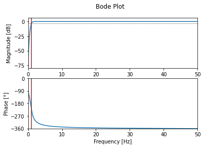
上面的代码,设计了一个采样频率100Hz,截止频率1Hz的高通滤波器。结果如下:
Coefficients b = [ 0.93909165 -2.81727496 2.81727496 -0.93909165] a = [ 1. -2.87435689 2.7564832 -0.88189313] |
滤波器的伯德图如下:
二、设计低通滤波器
与高通滤波器类似,python代码如下:
|
from scipy.signal import butter, freqz f_s = 100 # Sample frequency in Hz omega_c = 2 * pi * f_c # Cut-off angular frequency # Design the digital Butterworth filter w, H = freqz(b, a, 4096) # Calculate the frequency response # Plot the amplitude response # Plot the phase response plt.show() |
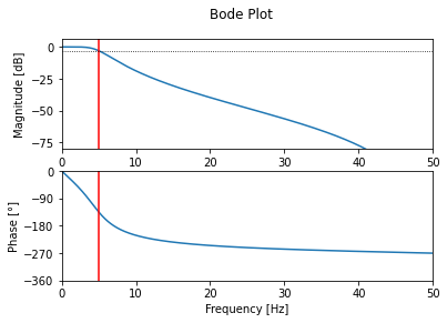
设计结果:
Coefficients b = [0.00289819 0.00869458 0.00869458 0.00289819] a = [ 1. -2.37409474 1.92935567 -0.53207537] |
伯德图:
三、如何写C代码
有了滤波器的a和b向量,就可以使用了。
IIR数字滤波器的一般形式:
y(n) = SUM(b[m]*x[m]) - SUM(a[n]*y[n])
其中,m从0到滤波器的阶数ORDER,n从1到ORDER。
具体代码如下:
低通滤波器
|
// cutoff 1Hz for (i=HPF_ORDER;i>0;i--){ //y(i)=b1*x(i)+b2*x(i-1)+b3*x(i-2)+b4*x(i-3)-a2*y(i-1)-a3*y(i-2)-a4*y(i-3); |
高通滤波器
|
// cutoff 5Hz for (i=LPF_ORDER;i>0;i--){ //y(i)=b1*x(i)+b2*x(i-1)+b3*x(i-2)+b4*x(i-3)-a2*y(i-1)-a3*y(i-2)-a4*y(i-3); |
带着使命来到世上的你,给他人提供价值,才有价值